Color-Guided Depth Recovery From RGB-D Data
Using an Adaptive Autoregressive Model
Jingyu Yang, Xinchen Ye, Kun Li, Chunping Hou, and Yao Wang
Abstract
This paper proposes an adaptive color-guided auto-regressive (AR) model for high quality depth recovery from low quality measurements captured by depth cameras. We observe and verify that the AR model tightly fits depth maps of generic scenes. The depth recovery task is formulated into a minimization of AR prediction errors subject to measurement consistency. The AR predictor for each pixel is constructed according to both the local correlation in the initial depth map and the nonlocal similarity in the accompanied high quality color image. We analyze the stability of our method from a linear system point of view, and design a parameter adaptation scheme to achieve stable and accurate depth recovery. Quantitative and qualitative results show that our method outperforms four state-of-the-art schemes. Being able to handle various types of depth degradations, the proposed method is versatile for mainstream depth sensors, ToF camera and Kinect, as demonstrated by experiments on real systems.
Keywords: Depth recovery (upsampling, inpainting, denoising), autoregressive model, RGB-D camera (ToF camera, Kinect)
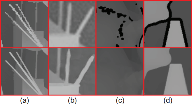
Fig. 1. Depth maps recovered by the proposed method from various types of degradations: (a) undersampling (1/8), (b) undersampling (1/8) with strong signal-dependent additive noise, (c) random missing, and (d) structural missing. The degraded depths and the recovered ones are at the top row and bottom row, respectively. The undersampled depths in (a) and (b) are enlarged with bicubic interpolation for illustration.
Downloads
Datasets: Various datasets can be downloaded via the links attached to the following tables and figures.
Source code: download here
Evaluation on Synthetic Datasets
1. Quantitative and Qualitative Results of Depth Upsampling
Table 1 : Quantitative upsamping results (in MAD) From undersampled depth maps on Middlebury datasets at four subsampling rates.
| Art | Book | Moebius | Reindeer | Laundry | Dolls | |||||||||||||||||||
| 2× | 4× | 8× | 16× | 2× | 4× | 8× | 16× | 2× | 4× | 8× | 16× | 2× | 4× | 8× | 16× | 2× | 4× | 8× | 16× | 2× | 4× | 8× | 16× | |
| Bicubic | 0.48 | 0.97 | 1.85 | 3.59 | 0.13 | 0.29 | 0.59 | 1.15 | 0.13 | 0.3 | 0.59 | 1.13 | 0.3 | 0.55 | 0.99 | 1.88 | 0.28 | 0.54 | 1.04 | 1.95 | 0.2 | 0.36 | 0.66 | 1.18 |
| MRF [1] | 0.59 | 0.96 | 1.89 | 3.78 | 0.21 | 0.33 | 0.61 | 1.2 | 0.24 | 0.36 | 0.65 | 1.25 | - | - | - | - | - | - | - | - | - | - | - | - |
| IMLS[2] | 0.27 | 0.68 | 1.04 | 2.2 | 0.16 | 0.26 | 0.48 | 1.16 | 0.15 | 0.25 | 0.49 | 0.93 | 0.32 | 0.64 | 0.74 | 1.43 | 0.23 | 0.39 | 0.81 | 1.53 | 0.24 | 0.36 | 0.61 | 0.98 |
| JBFcv[3] | 0.55 | 0.68 | 1.44 | 3.52 | 0.29 | 0.44 | 0.62 | 1.45 | 0.38 | 0.46 | 0.67 | 1.1 | - | - | - | - | - | - | - | - | - | - | - | - |
| Guided[4] | 0.63 | 1.01 | 1.7 | 3.46 | 0.22 | 0.35 | 0.58 | 1.14 | 0.23 | 0.37 | 0.59 | 1.16 | 0.42 | 0.53 | 0.88 | 1.8 | 0.38 | 0.52 | 0.95 | 1.9 | 0.28 | 0.35 | 0.56 | 1.13 |
| Edge [5] | 0.41 | 0.65 | 1.03 | 2.11 | 0.17 | 0.3 | 0.56 | 1.03 | 0.18 | 0.29 | 0.51 | 1.1 | 0.2 | 0.37 | 0.63 | 1.28 | 0.17 | 0.32 | 0.54 | 1.14 | 0.16 | 0.31 | 0.56 | 1.05 |
| PS[6] | - | 0.93 | - | - | - | 0.16 | - | - | - | 0.17 | - | - | - | 0.56 | - | - | - | 1.13 | - | - | - | 0.83 | - | - |
| CLMF0[7] | 0.43 | 0.74 | 1.37 | 2.95 | 0.14 | 0.28 | 0.51 | 1.06 | 0.15 | 0.29 | 0.52 | 1.01 | 0.32 | 0.51 | 0.84 | 1.51 | 0.3 | 0.5 | 0.82 | 1.66 | 0.24 | 0.34 | 0.66 | 1.02 |
| CLMF1[7] | 0.44 | 0.76 | 1.44 | 2.87 | 0.14 | 0.28 | 0.51 | 1.02 | 0.15 | 0.29 | 0.51 | 0.97 | 0.32 | 0.51 | 0.84 | 1.55 | 0.3 | 0.5 | 0.8 | 1.67 | 0.23 | 0.34 | 0.6 | 1.01 |
| JGF[8] | 0.29 | 0.47 | 0.78 | 1.54 | 0.15 | 0.24 | 0.43 | 0.81 | 0.15 | 0.25 | 0.46 | 0.8 | 0.23 | 0.38 | 0.64 | 1.09 | 0.21 | 0.36 | 0.64 | 1.2 | 0.19 | 0.33 | 0.59 | 1.06 |
| TGV[9] | 0.45 | 0.65 | 1.17 | 2.3 | 0.18 | 0.27 | 0.42 | 0.82 | 0.18 | 0.29 | 0.49 | 0.9 | 0.32 | 0.49 | 1.03 | 3.05 | 0.31 | 0.55 | 1.22 | 3.37 | 0.21 | 0.33 | 0.7 | 2.2 |
| Ours_FP[10] | 0.18 | 0.49 | 0.66 | 2.15 | 0.12 | 0.25 | 0.48 | 0.8 | 0.11 | 0.25 | 0.42 | 0.9 | 0.22 | 0.4 | 0.64 | 1.21 | 0.2 | 0.35 | 0.59 | 1.2 | 0.21 | 0.36 | 0.56 | 1.09 |
| Ours_AP | 0.18 | 0.49 | 0.64 | 2.01 | 0.12 | 0.22 | 0.37 | 0.77 | 0.1 | 0.2 | 0.4 | 0.79 | 0.22 | 0.4 | 0.58 | 1 | 0.2 | 0.34 | 0.53 | 1.12 | 0.21 | 0.34 | 0.5 | 0.82 |
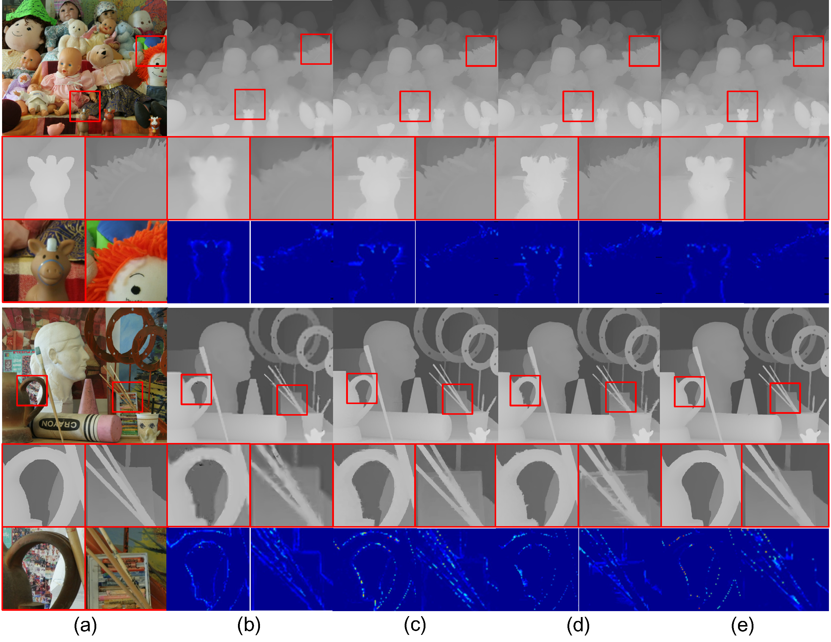
Fig.2. Visual quality comparison for depth upsampling on Middlebury RGB-D pairs: (a) color image and depth ground truth, depth maps upsampled (8×)
by (b) IMLS [2] (MAD: 0.61; 1.04), (c) EDGE [5] (MAD: 0.56; 1.03), (d) JGF [8] (MAD: 0.59; 0.78), and (e) our method (MAD:
0.50; 0.64). The first and second MADs for each method are for Dolls and Art, respectively.
2.Quantitative and Qualitative Results on ToF-like Depth Degradations
Table 2 : Quantitative depth recovery results from ToF-like degradations (undersampling with noise) at four subsampling rates.
| Art | Book | Moebius | Reindeer | Laundry | Dolls | |||||||||||||||||||
| 2× | 4× | 8× | 16× | 2× | 4× | 8× | 16× | 2× | 4× | 8× | 16× | 2× | 4× | 8× | 16× | 2× | 4× | 8× | 16× | 2× | 4× | 8× | 16× | |
| Bicubic | 3.52 | 3.84 | 4.47 | 5.72 | 3.3 | 3.37 | 3.51 | 3.82 | 3.28 | 3.36 | 3.5 | 3.8 | 3.39 | 3.52 | 3.82 | 4.45 | 3.35 | 3.49 | 3.77 | 4.35 | 3.28 | 3.34 | 3.47 | 3.72 |
| IMLS[2] | 1.43 | 1.95 | 3.37 | 4.67 | 0.81 | 1.39 | 2.68 | 3.21 | 0.87 | 1.4 | 2.65 | 3.16 | 0.92 | 1.49 | 2.86 | 3.53 | 0.94 | 1.53 | 2.83 | 3.58 | 0.81 | 1.34 | 2.57 | 3.09 |
| Guided[4] | 1.49 | 1.97 | 3 | 4.91 | 0.8 | 1.22 | 1.95 | 3.04 | 1.18 | 1.9 | 2.77 | 3.55 | 1.29 | 1.99 | 2.99 | 4.14 | 1.28 | 2.05 | 3.04 | 4.1 | 1.19 | 1.94 | 2.8 | 3.5 |
| Edge[5] | 1.69 | 2.4 | 3.6 | 5.75 | 1.12 | 1.44 | 1.81 | 2.59 | 1.13 | 1.45 | 1.95 | 2.91 | 1.2 | 1.6 | 2.4 | 3.97 | 1.28 | 1.63 | 2.2 | 3.34 | 1.14 | 1.54 | 2.07 | 3.02 |
| PS[6] | - | 1.46 | - | - | - | 1.09 | - | - | - | 1.17 | - | - | - | 1.21 | - | - | - | 1.53 | - | - | - | 1.33 | - | - |
| CLMF0[7] | 1.19 | 1.77 | 2.95 | 4.91 | 0.9 | 1.48 | 2.38 | 3.36 | 0.87 | 1.44 | 2.32 | 3.3 | 0.96 | 1.56 | 2.54 | 3.85 | 0.94 | 1.55 | 2.5 | 3.81 | 0.96 | 1.54 | 2.37 | 3.25 |
| JGF[8] | 2.36 | 2.74 | 3.64 | 5.46 | 2.12 | 2.25 | 2.49 | 3.25 | 2.09 | 2.24 | 2.56 | 3.28 | 2.18 | 2.4 | 2.89 | 3.94 | 2.16 | 2.37 | 2.85 | 3.9 | 2.09 | 2.22 | 2.49 | 3.25 |
| TGV[9] | 0.82 | 1.26 | 2.76 | 6.87 | 0.5 | 0.74 | 1.49 | 2.74 | 0.56 | 0.89 | 1.72 | 3.99 | 0.59 | 0.84 | 1.75 | 4.4 | 0.61 | 1.59 | 1.89 | 4.16 | 0.66 | 1.63 | 1.75 | 3.71 |
| Ours_AP | 0.76 | 1.01 | 1.7 | 3.05 | 0.47 | 0.7 | 1.15 | 1.81 | 0.46 | 0.72 | 1.15 | 1.92 | 0.48 | 0.8 | 1.29 | 2.02 | 0.51 | 0.85 | 1.3 | 2.24 | 0.59 | 0.91 | 1.32 | 2.08 |

Fig. 3. Visual quality comparison for recovered depth maps from ToF-like degradation mode (8×upsampling with intense Gaussian noise): depth maps are recovered by (a) Bicubic (MAD: 3.51; 3.82), (b) IMLS [2] (MAD: 2.68; 2.86), (c) EDGE [5] (MAD: 2.07; 3.60), (d) TGV [9] (MAD: 1.49; 1.75), and (e) our method (MAD: 1.15; 1.29). The two MADs for each method are for Book (first) and Reindeer (second) respectively. For visual inspection, the error maps are shown by subtracting between recovered depth and ground truth.
3.Quantitative and Qualitative Results for Kinect-like Depth Degradations
Table 3 : Quantitative depth recovery results from Kinect-like degradations (structural missing and random missing) .
| Bicubic | 0.9 |
0.61 |
0.66 |
0.95 |
0.91 |
0.76 |
| IMLS[2] | 0.91 |
0.58 |
0.72 |
0.68 |
0.72 |
0.82 |
| JBF[11] | 0.84 |
0.63 |
0.69 |
0.92 |
0.88 |
0.76 |
| Guided[4] | 1.2 |
0.63 |
0.67 |
0.96 |
0.94 |
0.76 |
| CLMF0[7] | 1.01 |
0.6 |
0.64 |
0.94 |
0.89 |
0.74 |
| Ours_AP | 0.58 |
0.53 |
0.6 |
0.68 |
0.75 |
0.69 |
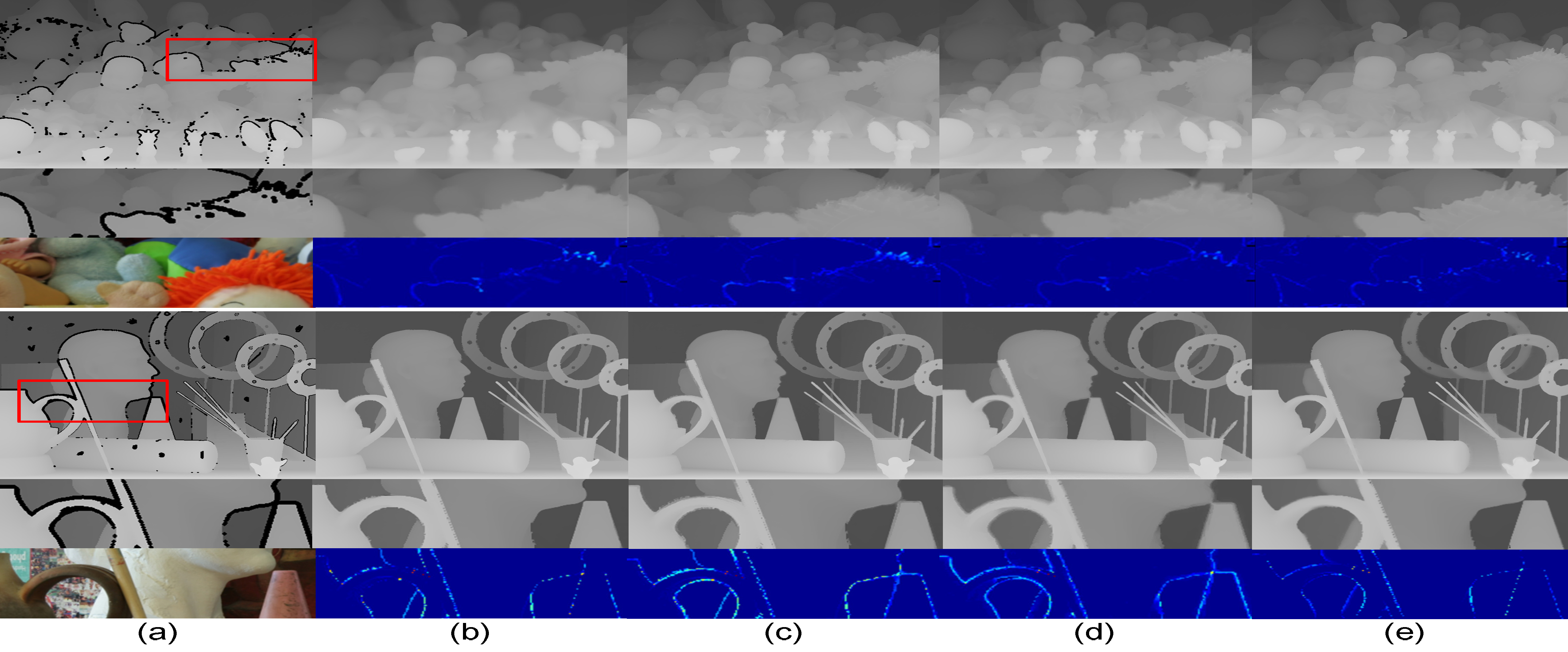
Fig. 4. Visual quality comparison for recovered depth maps from Kinect-like degradation mode: (a) degraded depth map, depth maps recovered by
(b) IMLS [2] (MAD: 0.76; 0.90), (c) JBF [11] (MAD: 0.76; 0.84), (d) CLMF0 [7] (MAD: 0.74; 1.01), and (d) our method
(MAD: 0.69; 0.58). The MADs for each method are for Art. For visual inspection, regions highlighted by rectangles are enlarged, and the error maps are shown
by subtracting between recovered depth and ground truth.
Evaluation on Real Datasets
1.ToF Depth Maps

Fig. 5. Depth recovery results for the depth-color camera rig in Fig. 12: (a) RDB-D pairs, recovered depth maps by (b)multipoint filtering (CLMF0) [7], (c) geodesic upsampling [8], (d) IMLS [2], and (e) our method. Captured depth maps are overlaid on the color images to save space. Regions highlighted by red rectangles are enlarged for better visual inspection.
Click here to download all the pictures in Fig.5.
Table 4: Quantitative depth upsampling results for ToFmark datasets.
| Bicubic | IMLS[2] | JBF[11] | Guided[4] | CLMF0[7] | JGF[8] | TGV[9] | Ours | |
| Books | 16.23 | 14.5 | 16.03 | 15.74 | 13.89 | 17.39 | 12.36 | 12.25 |
| Shark | 17.78 | 16.26 | 18.79 | 18.21 | 15.1 | 18.17 | 15.29 | 14.71 |
| Devil | 16.66 | 14.97 | 27.57 | 27.04 | 14.55 | 19.02 | 14.68 | 13.83 |
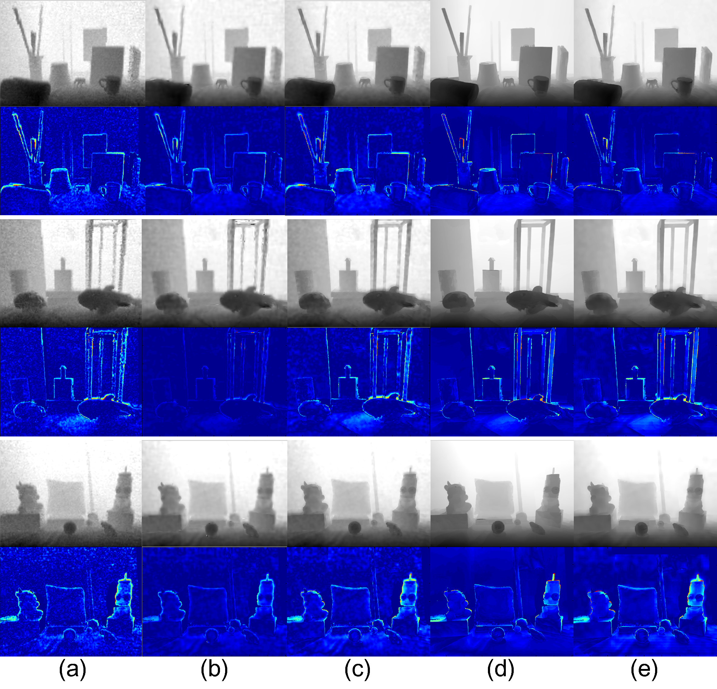
Fig. 6. Visual quality comparison on depth recovery for Books, Shark, Devil from ToFmark datasets [14]: (a) Bicubic, (b) IMLS [2], (c) CLMF0[7], (d)TGV [9], and (e) our method. For visual inspection, the error maps are shown by subtracting between recovered depth and ground truth.
2.Kinect Depth Maps

Fig.7. Depth recovery results for RGB-D pairs captured by Kinect: (a) RDB-D pairs, recovered depth maps by (b) IMLS [2], (c) joint multilateral filtering [12], and (d) our method. Regions highlighted by red rectangles are enlarged for better visual inspection. RGB-D pairs in (a)-(c) are from the NYU RGB-D dataset [13], while the rest two are captured in our lab.
Click here to download all the pictures in Fig.7.
1. Jingyu Yang, Xinchen Ye, Kun Li, Chunping Hou, Yao Wang, “Color-Guided Depth Recovery From RGB-D Data Using an Adaptive Autoregressive Model”, IEEE Transactions on Image Processing, vol. 23, no. 8, pp. 3443-3458, 2014. [pdf][bib]
2. Jingyu Yang, Xinchen Ye, Kun Li, and Chunping Hou, “Depth recovery using an adaptive color-guided auto-regressive model”, European Conference on Computer Vision (ECCV), ....October 7-13, 2012, Firenze, Italy. [pdf] [bib]
[1] J. Diebel, S. Thrun, “An application of Markov random fields to range sensing,” Advances in Neural Information Processing Systems, p. 291, 2005.
[2] N. K. Bose and N. A. Ahuja, “Superresolution and noise filtering using
moving least squares,” IEEE TIP, vol. 15, no. 8, pp. 2239–2248, 2006.
[3] Q. Yang, R. Yang, J. Davis, and D. Nistér, “Spatial-depth super resolution for range images,” in Proc. IEEE CVPR, 2007, pp. 1–8.
[4] K. He, J. Sun, and X. Tang, “Guided image filtering,” in Proc. ECCV, 2010, pp. 1–14.
[5] J. Park, H. Kim, Y.-W. Tai, M. S. Brown, and I. Kweon, “High quality depth map upsampling for 3D-TOF cameras,” in Proc. IEEE ICCV, 2011.
[6] O. Mac Aodha, N. D. Campbell, A. Nair, and G. J. Brostow, “Patch based synthesis for single depth image super-resolution,” in ECCV 2012, pp. 71–84.
[7] J. Lu, K. Shi, D. Min, L. Lin, and M. N. Do, “Cross-based local multipoint filtering,” in Proc. IEEE CVPR, 2012, pp. 430–437.
[8] M.-Y. Liu, O. Tuzel, and Y. Taguchi, “Joint geodesic upsampling of depth images,” in Proc. IEEE CVPR, 2013, pp. 169–176.
[9] D. Ferstl, C. Reinbacher et.al., “Image guided depth upsampling using anisotropic total generalized variation.” in Proc. IEEE ICCV, 2013.
[10] J. Yang, X. Ye, K. Li, and C. Hou, “Depth recovery using an adaptive color-guided auto-regressive model,” in Proc. ECCV, 2012, pp. 158–171.
[11] A. Riemens, O. Gangwal, B. Barenbrug, and R. Berretty, “Multi-step joint bilateral depth upsampling,” in Proc. of SPIE VCIP, 2009, pp. 1–12.
[12] S. Lee and Y. Ho, “Joint multilateral filtering for stereo image generation
using depth camera,”The Era of Interactive Media, pp. 373–383, 2013.
[13] NYU datasets, “http://cs.nyu.edu/~silberman/datasets/.”
[14] ToFmark datasets, “http://rvlab.icg.tugraz.at/tofmark/.”
